Session 3 · Visualisation

The term-object API loads skeletons and plots them co-registered in a chosen template space — navis under the bonnet.

from vfb_connect import vfb

da1 = vfb.term("VFB_jrchjtdb")
da1.load_skeleton(template="JRC2018Unisex")
print(da1.skeleton)                     # TreeNeuron, 4847 nodes (verified)

# interactive 3D over the standard template (in a notebook / Colab)
da1.plot3d(template="JRC2018Unisex", include_template=True)

# overlay its strongest partners in the same space
partners = da1.downstream_partners(weight=30)
da1.plot_partners(partners[:3], template="JRC2018Unisex")

Always pass the template explicitly — that is what guarantees every neuron you add is in the same coordinate space, whichever dataset it came from. plot2d() gives a publication-ready still with the same arguments.

The term-object API works through reticulate too — skeletons load as navis objects, and nat users can pull them natively instead.

da1 <- vfb$term("VFB_jrchjtdb")
da1$load_skeleton(template = "JRC2018Unisex")
da1$skeleton                       # navis TreeNeuron, 4847 nodes (verified)
da1$plot3d(template = "JRC2018Unisex", include_template = TRUE)

For a fully native R workflow, vfbconnectr::read.neurons.vfb("VFB_jrchjtdb", template = "JRC2018Unisex") returns a nat::neuronlist, so plot3d() from nat/rgl and the whole natverse toolchain apply. Either way, pass the template explicitly — that is what keeps every neuron in the same coordinate space.

get_term_info returns the registered images for a neuron keyed by template brain — and the MCP documents how to turn those into a live 3D scene URL, so your assistant can hand you a clickable view:

You: Show me neuron VFB_jrchjtdb in 3D and summarise what it is.

Assistant → get_term_info(VFB_jrchjtdb) → images aligned to JRCFIB2018Fum (VFB_00101384) and JRC2018Unisex (VFB_00101567); classification, predicted transmitter, lineage

Assistant: DA1_lPN_R (FlyEM-HB:1734350908) is an adult antennal lobe projection neuron DA1 lPN (also typed adult fruitless aDT-e (female) neuron), lineage ALl1/BAlc, predicted cholinergic (91%, connectome data). View it in 3D over the standard JRC2018Unisex template: https://v2.virtualflybrain.org/org.geppetto.frontend/geppetto?id=VFB_jrchjtdb&i=VFB_00101567,VFB_jrchjtdb — swap the first ID in i= to VFB_00101384 to see it over its native hemibrain EM volume instead.

Download formats (SWC, OBJ, NRRD) are listed per image, so “get me the skeleton file” is also one question away.

Chat can help you find neurons to visualise, though for publication-quality figures you’ll want the Python API.

Optimized prompt: Ask by the neuron’s name for its images plus key facts in one question.

This is the browser’s home ground: publication-quality sanity-checking with zero installs.

1. Load neurons. Run any image query (see Session 1) and tick the checkboxes of the neurons you want — here the left and right Male CNS DA1 lPNs — or open the pre-built scene with the button below.

2. Drive the scene. Each neuron gets a colour and a row in the Layers panel: click the eye to hide/show, the swatch to recolour, the name to bring up its Term Info. The template brain stays as anatomical context, and the Slice Viewer tracks the same alignment so you can flick between 3D and section views.

   

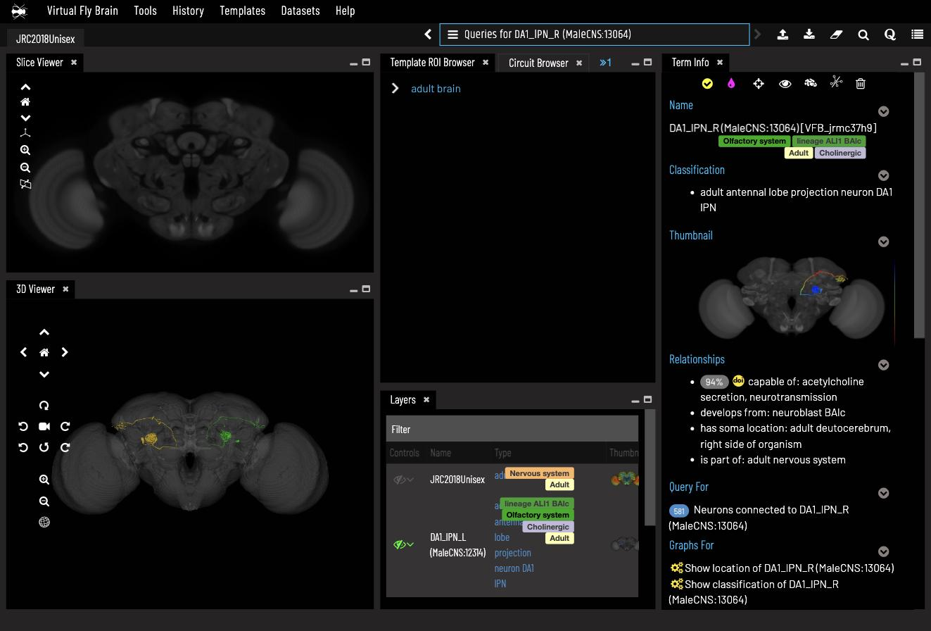
3. Interrogate any neuron. With an individual selected, Term Info shows its neurotransmitter prediction (94% acetylcholine here), soma side, lineage — and one-click queries such as Neurons connected to….

4. Share the exact view. The URL updates as you work: it records the template and every loaded neuron. Copy it into a paper, a Slack message or a lab notebook and anyone opens the identical scene — that is what the button below does.

Worth noticing: stick to the standard JRC2018Unisex space for comparisons — but if you open an EM neuron with its native template first in i= (e.g. ?id=VFB_jrchjtdb&i=VFB_00101384,VFB_jrchjtdb), the raw hemibrain EM volume loads behind the skeleton and you can scroll the actual electron microscopy it was traced from.