Session 7 · Putting It Together

The whole chain with the term-object API — every step verified live (Aug 2026), IDs carried forward throughout.

from vfb_connect import vfb

# 1. Region → intrinsic types (the ontology knows the answer)
kc_types = vfb.term("Kenyon cell").children          # 37 subtypes

# 2. Type → instances; pick one with connectome data
inst = vfb.get_instances("alpha/beta Kenyon cell", return_dataframe=True)
print(len(inst), "records")                          # 7212
hb = inst[inst.data_source.astype(str).str.contains('hb')]
kc = vfb.term(hb['id'].iloc[0])                      # e.g. KCab-m_R

# 3. Visualise in the standard space
kc.load_skeleton(template="JRC2018Unisex")
kc.plot3d(template="JRC2018Unisex", include_template=True)

# 4. Strongest partners
for p in kc.downstream_partners(weight=20):
    print(p)

# 5. Cross-dataset matches
m = vfb.get_similar_neurons(kc.id, similarity_score='NBLAST_score',
                            return_dataframe=True)

# 6. Expression
e = vfb.get_transcriptomic_profile("alpha/beta Kenyon cell",
                                   return_dataframe=True)   # 18234 rows

Verified payoff at step 4 — the Kenyon cell’s strongest partners are exactly the mushroom-body cast you would hope for:

Partner(weight=34, partner=APL_R (FlyEM-HB:425790257))
Partner(weight=31, partner=DPM_R (FlyEM-HB:5813105172))
Partner(weight=23, partner=MBON06(B1>a)(AVM07)_L (FlyEM-HB:422725634))

The giant inhibitory APL, the modulatory DPM, and an MBON — the textbook mushroom-body circuit, recovered from a cold start in six calls.

The full chain, verified in R (identical results to the Python route):

library(reticulate)
vfb <- import("vfb_connect")$vfb

kc_types <- vfb$term("Kenyon cell")$children               # 37 subtypes
inst <- vfb$get_instances("alpha/beta Kenyon cell",
                          return_dataframe = TRUE)         # 7212 records
hb  <- inst[grepl("hb", sapply(inst$data_source, paste, collapse=",")), ]
kc  <- vfb$term(hb$id[[1]])                                # e.g. KCab-m_R

kc$load_skeleton(template = "JRC2018Unisex")
kc$plot3d(template = "JRC2018Unisex", include_template = TRUE)

for (p in kc$downstream_partners(weight = 20L)) print(p)
m <- vfb$get_similar_neurons(kc$id, similarity_score = "NBLAST_score",
                             return_dataframe = TRUE)
e <- vfb$get_transcriptomic_profile("alpha/beta Kenyon cell",
                                    return_dataframe = TRUE)

Verified payoff — the same textbook mushroom-body cast as the Python route:

Partner(weight=34, partner=APL_R (FlyEM-HB:425790257))
Partner(weight=31, partner=DPM_R (FlyEM-HB:5813105172))
Partner(weight=23, partner=MBON06(B1>a)(AVM07)_L (FlyEM-HB:422725634))

From here the natverse is one step away: pull the same IDs with vfbconnectr::read.neurons.vfb() and continue in nat.

With the MCP connected, the whole chain is one conversation — the assistant carries the IDs forward so every step is reproducible. A real end-to-end transcript, condensed:

You: Starting from the mushroom body: find its intrinsic neuron types, pick one, show it, list its main partners, find its closest match in another connectome, and summarise any expression data — give me all the VFB IDs.

Assistant → search_terms("mushroom body") → FBbt_00005801 get_term_info(FBbt_00005801) → queries incl. NeuronsPartHere (602), PartsOf (176), TransgeneExpressionHere (4130) get_hierarchy("mushroom body intrinsic neuron", subclass_of) → Kenyon cell (FBbt_00003686) and its 37 subclasses run_query(FBbt_00003686, ListAllAvailableImages) → 32,328 records → picks a hemibrain KC with images run_query(<KC id>, NeuronNeuronConnectivityQuery) → ranked partners with synapse counts run_query(<KC id>, SimilarMorphologyTo) → cross-dataset NBLAST matches run_query(FBbt_00003686, anatScRNAseqQuery) → 79 clusters with publications

Assistant: …a summary with every claim carrying a VFB ID, dataset and (for expression) a PMID — paste the IDs straight into vfb_connect to reproduce the analysis in Python.

The pattern to copy: resolve the name to an ID first, then let each result’s IDs seed the next question. That is exactly what the Python route does — the MCP just lets your assistant drive it.

Walk through the same chain one question at a time in chat. Each question builds on the previous answer.

Step-by-step prompts:

1. “What neuron types are intrinsic to the mushroom body?”
2. “Show me instances of Kenyon cell with VFB IDs.”
3. “What are the top 5 downstream partners of KCg-m_R?”
4. “Which neurons have a similar morphology to KCg-m_R?”
5. “What expression data exists for Kenyon cells?”

Use the names the chat itself uses in its answers — plain names resolve better than IDs pasted into long questions.

The whole Session 1→Session 6 chain works as one browsing session — every answer is a link to the next question, and the History menu retraces your steps.

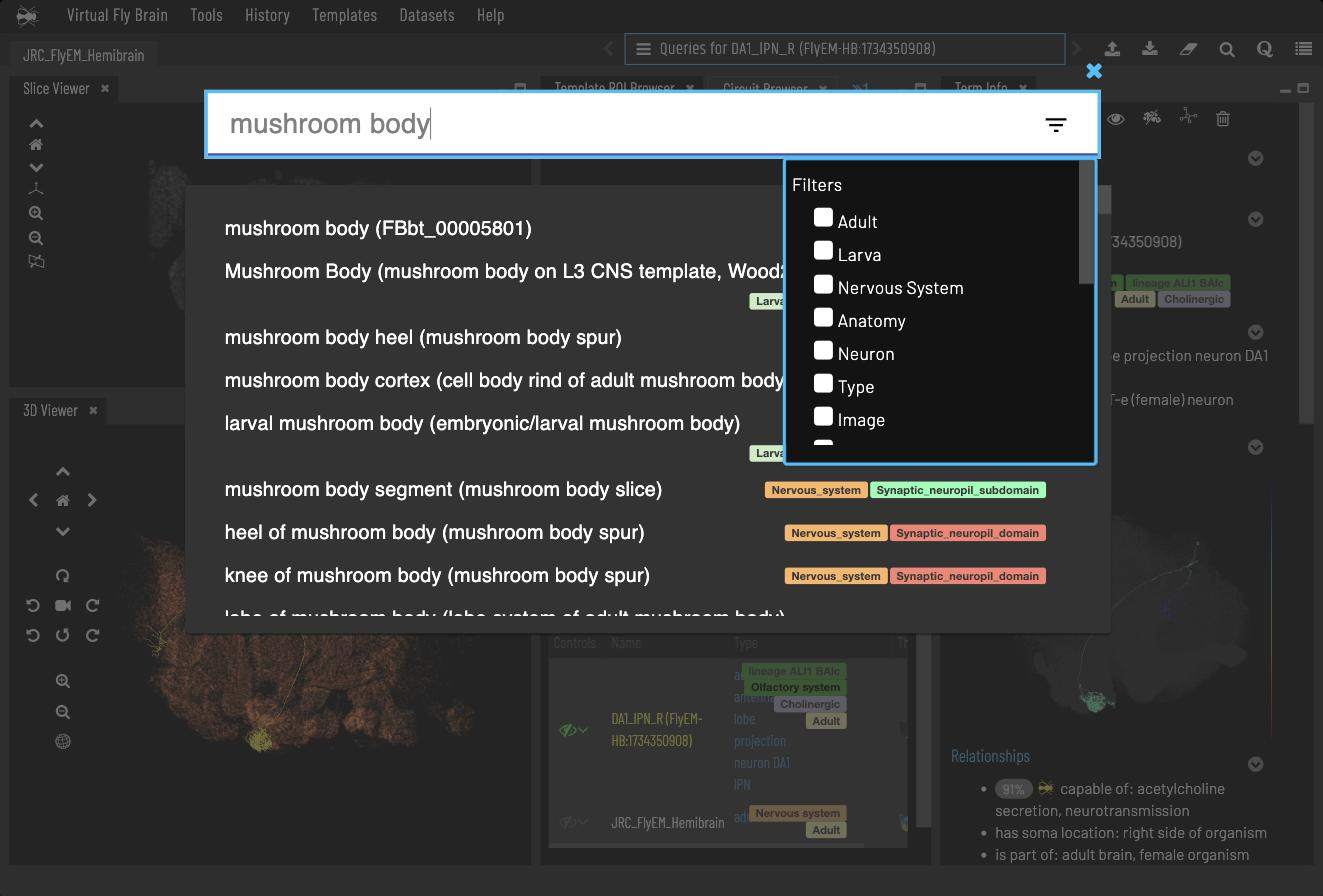
1. Start from the region. Search mushroom body — the suggestion list’s facet tags already separate the neuropil, its parts and its larval counterpart. Pick mushroom body (FBbt_00005801).

   

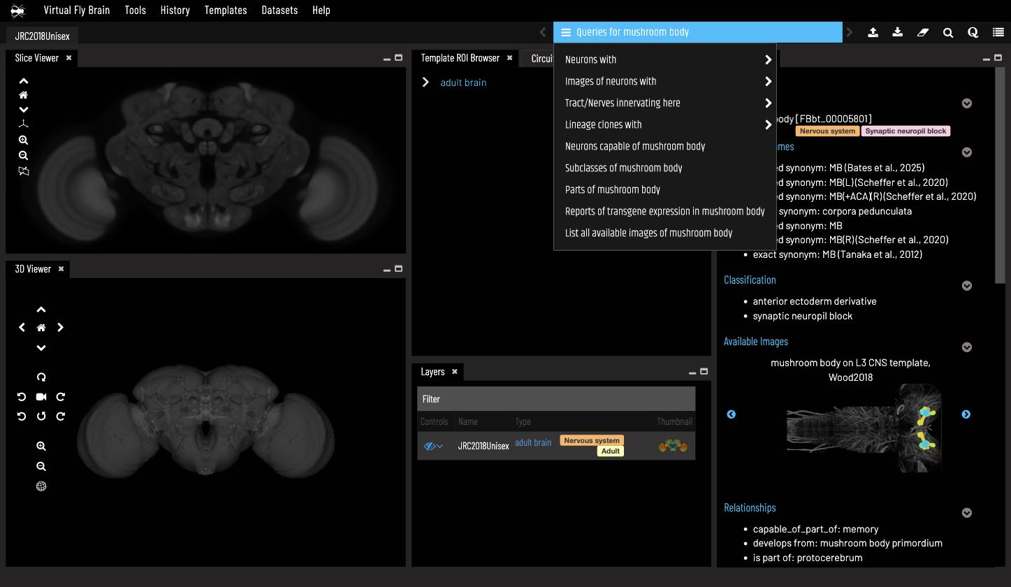
2. Survey what VFB can tell you. The region’s query menu is the whole workshop in miniature: Neurons with ▸ (innervating here), Tract/Nerves innervating here, Lineage clones, Subclasses, Parts of mushroom body, Reports of transgene expression, and List all available images.

   

3. Region → type. Run Neurons with ▸ some part here and pick a Kenyon cell from the results — or go via Parts of mushroom body to the calyx and its intrinsic neurons.

4. Type → instance → partners. From the Kenyon cell’s term page, list its images (Session 1), tick one into the 3D viewer (Session 3), and run Neurons connected to… on it (Session 4).

5. Instance → matches → expression. NBLAST its neighbours (Session 5), then check Reports of transgene expression for the type (Session 6).

6. Keep the trail. The History menu (top bar) lists every term and query you touched, and the final URL encodes your finished scene — paste it anywhere to hand a colleague your entire session.

Worth noticing: you never typed an ID. The graph carried you from a word (“mushroom body”) to specific, citable individuals with IDs — which is exactly what you then feed to vfb_connect to make it reproducible.